While parts of the world today are experiencing water shortages of varying severity, numerical assessments on the current state of water across the globe are disorganized at best and absent at worst. The integrative nature of water at a political, economic, and social level as well as the enormous volumes used daily makes its usage difficult to measure and even harder to project, resulting in sparse data collection and models that are either inaccurate or too complex for easy use [1]. The task of finding convincing evidence to support water policy, infrastructure, and technology changes remains a large obstacle in easing and averting water crises.
Mission 2017 has developed a model for projecting changes in water demand by country, with the goal of illustrating the complexity of water usage, the cost of inaction, and the urgency with which solutions must be implemented. The model integrates several measures of development from idealized future scenarios predicted by the UN, World Bank, and other organizations, in which each country experiences steady and unimpeded growth, but does not make any substantial efforts towards water conservation and more efficient water use. The model illustrates the unsustainability of status quo water usage and perspectives and the extent of water stress in the future when following a global “best-case scenario.”
Discussed in this article is the determination of important predictive variables, justification of mathematical models used, assessment of the model against real data, water demand projections to 2030, observations on a global scale, and the model as a basis for understanding how to approach the water crisis.
Choosing Predictive Variables
Projections were developed by comparing several variables known to be linked to water usage to actual historic water usage data, at a country-by-country basis. Specifically, the model estimates an internal water demand defined as the total amount of water used within a country, excluding water demanded through imports in the form of “virtual water” (water consumed to create a product, such as for irrigation and processing of food products). While there exist numerous such predictive variables, many of these variables are interconnected and not well understood; a model that incorporates dozens of such variables would only offer slight improvements in accuracy than one that incorporates a few inherently different variables, and would be much more difficult to interpret.
Mission 2017 has limited the scope of the model to quantities that are largely independent and have been best analyzed and projected at a country scale by previous studies. Specifically, the model integrated predictive measures studied in the World Resource Institute (WRI) Aqueduct Atlas study [2], physical factors from the United Nations’ Food and Agriculture Organization (FAO) Irrigation Guidelines [3], and variables Missions 2017 hypothesized to be linked to an overall measure of “development” as referenced in MIT’s study on water resources [1]. All data was taken from the World Bank Database [4], unless otherwise specified. In total, the variables considered by the model were:
- Population
- Gross Domestic Product
- Total energy consumption, from EIA [5]
- Life expectancy estimates, from UN [6]
- Agricultural land area
- Annual temperature average
- Annual precipitation average
Details on their usage are in subsequent sections.
Model Design
The model was designed with the goal of determining a relationship between the predictive variables and water withdrawal, or amount of freshwater pulled from natural water stores (rivers, reservoirs, groundwater, etc.). Water demand was analyzed separately for each of FAO’s AQUASTAT’s (database of international water resources and usage) three sectors for water withdrawal, defined as [7]:
- Municipal: ”Water withdrawn primarily for the direct use by the population.”
- Industrial: “Water withdrawn for industrial uses… refers to self-supplied industries not connected to the public distribution network.”
- Agricultural: “Water withdrawn for irrigation, livestock and aquaculture purposes.”
Mission 2017 used these divisions in order to better understand sources for water demand, as each sector uses water for inherently different means. Additionally, the divisions were maintained to make better use of water withdrawal data, which is frequently disaggregated into these sectors [7].
In projecting future water demand, the model uses values for the predictive variables as projected in future global scenarios from other studies. In adhering to these scenarios, the model does not take into account the feedback effect of increasing water demand on the predictive variables. Rather, the model focuses on the unsustainability of current global water usage when extrapolating along these scenarios.
The Consumer, Development, and Water Demand
The model was developed with an emphasis on determining by sector, who the main consumers of water are, how to measure development, and how a country’s level of development impacts how efficiently water is used. Quantitatively, the number of consumers is abbreviated as CSM, and the level of consumer development as DEV, where their definitions and effects vary by sector, as explained below. The model captures two main ideas with regard to consumers and development:
- The water demand is directly proportional to the number of consumers, or water demand is linear to CSM.
- MIT’s 2011 study of water resources states that, “The general pattern observed is that water requirements grow as a nation industrializes and then slows or even declines at higher levels of development with changing structure of industry and policies that lead to greater water reuse, recycling” [1]. Mission 2017 interprets the observation about development as water demand per consumer increases with development up to a certain point, after which further development decreases water demand per consumer (economic forces drive improvements in efficiency, including water use).
To capture the effect of development mathematically, we used product of a linear function and a slowly decaying exponential of DEV. This model was chosen for its simplicity, ability to capture the effects mentioned above, and realistic behavior at both extremes of development. The function is presented below:
Combining both of the effects of CSM and DEV, the model’s equation for water use becomes:

Interpreting Consumer and Development
For municipal water use, CSM was set to population, as the main consumer of municipal water is the general population. For industrial water use, the proxy value of total energy consumption was used, as industrial energy consumption is nearly linear to total energy consumption [8] and is a rough measure of industrial activity. For agricultural water use, CSM was set to total agricultural land, measuring the area of land that incurs water demand for cultivation.
DEV for the municipal sector was interpreted as the state of municipal water distribution, in terms of both water access and distribution efficiency. Following the shape of the function, an under-developed state would have low usage as little to no water could be distributed, a developing state would have high usage as water would be distributed to a larger population but with poor efficiency, and a highly developed state would have decreasing usage as distribution efficiency and water recycling would increase. Mission 2017 makes the assumption that this measure of water distribution and availability is correlated to standard of living, taken as the product of GDP/capita (as an approximation for spending power per person) and life expectancy.
DEV for the industrial sector was interpreted as a level of technological development. Reasoning with the function, a technologically underdeveloped industry would have limited productivity, and would not be able to process as much input including water, a developing industry would be more productive and be able to process more input and water, and a highly developed industry would be more efficient with inputs. Technological development was modeled as GDP/capita, in which higher GDP/capita would correspond to higher productivity per person enabled by more advanced technology. While more sophisticated measures of development were available, the model was developed to make use of quantities that have been investigated and projected in detail in other studies.
Agricultural water use was analyzed differently as the effects of DEV, the development of the consumer, do not follow the same pattern as those of the other two sectors. FAO’s study on changes on agricultural land use states that by 2050, developing countries will experience an 80 percent increase in cropping intensity (percent of cultivated land actually harvested) and an 11 percent increase in irrigation equipped land, while developed countries will experience a 90 percent increase cropping intensity with no significant change in irrigation equipped land [9]. Since changes in cropping intensity is roughly proportional to changes in water need to grow larger quantities of food and irrigation was defined as the primary use of agricultural water, the combined effect of the 80 percent growth in cropping intensity and 11 percent growth in irrigated land corresponds to a 99 percent growth in water demand. Since the difference between 99 percent growth in developing countries and 90 percent growth in developed countries is small, agricultural water demand was modeled without DEV.
The agricultural water demand model also included temperature and precipitation, both factors described to have an approximately linear effect on irrigation requirements in FAO’s Irrigation Guidelines [3].
Additionally, in order to condense values of GDP/capita that spanned many orders of magnitude across all countries, DEV was taken as the logarithm of their corresponding development measures. Overall, the model’s equations are:
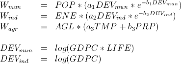
Where (a1,b1), (a2,b2), (a3,b3) are coefficients used to calibrate the model to real world data, and the predictive variables have been abbreviated as:
- POP = Population
- ENE = Total energy consumption
- AGL = Total agricultural land
- TMP = Average annual temperature
- PRP = Average annual precipitation
- GDPC = Gross domestic product per capita
- LIFE = Life Expectancy
Calibrating Model and Assessing Performance
Taking the above forms for the relationship between the predictive variables and water, the model creates useful equations for projecting demand by calibrating the coefficients to real world data. For a given set of historic values for the predictive variables, values for the coefficients were determined such that the model’s estimates for water demand match up best with historic water withdrawal data, or amount of freshwater pulled from natural water stores (rivers, reservoirs, groundwater, etc.) taken from FAO AQUASTAT [7].
Specifically, numeric values for coefficient pairs (a1,b1), (a2,b2), (a3,b3) for the equations for municipal, industrial, and agricultural water demand, respectively, were determined by minimizing the error function below:

Where, for each sector, PRD is the model’s estimated water demand from values of the predictive variables in a given country and year, and OBS is the observed water withdrawal for that country and year. In order to give equal attention to smaller countries, the error for each water withdrawal data point was calculated from the ratio between PRD and OBS, to assess how well the the model predicts the magnitude of a country’s water demand. The square of the logarithm was used to account for error from both undershooting and overshooting water demand.
While originally intended to model each country separately, given the limited amount of data available on water withdrawal (typically one or two data points per sector per country over the period 1970-2011 [1][7]), such models would be meaningless as there would be little to no data with which to test the model for its accuracy. Consequently, the model was calibrated using data across all countries, and the usefulness of the model’s equations when generalized across the world. Historic data for the predictive variables and observed water withdrawals was divided into two time groups, 1970-1990 and 1991-2011, in which the model was calibrated to the former and tested against the latter. By comparing recent observed data to those predicted by the model calibrated to older data, the model’s ability to predict future water demand can be assessed.
After optimizing the coefficients, a multiplicative bias for each country and sector was calculated as a geographic correction to better fit the input data (1970-1990). For each data point, a bias ratio was calculated as OBS/PRD and was associated with each country. For countries with multiple data points, the bias ratio was taken as the geometric mean of all OBS/PRD ratios.
The bias ratio for each country can be interpreted as a factor that accounts for roughly time-independent, country-specific variations that may not be covered by variations in the time-dependent predictive variables. By sector, sources for geographic bias covered by this correction include:
- Municipal: Distances between populated regions and water resources/efficiency in distribution, diet of population.
- Industrial: Ratio of proxy value “energy consumption” to actual industrial productivity, types of industries per country/composition of industrial sector.
- Agricultural: Soil texture and infiltration rates of cultivated areas, climatic zone, dominant crops grown per country, ratio between rainfed and irrigated farmland [3].
To assess the model’s performance, the coefficients and bias ratios calculated from the 1970-1990 data set were used to predict water demand by sector for the 1991-2011 data set. Values for CSM and DEV in the timescale of the second set were used to estimate values for water demand using the calibrated equations, which were then multiplied by the appropriate bias ratio by country and sector. A linear regression was conducted between the logarithm of predicted values and the logarithm of observed values as an assessment of how accurately the model estimated the water demand per country.
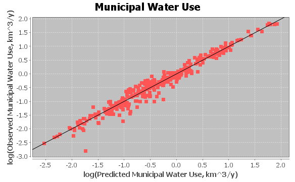

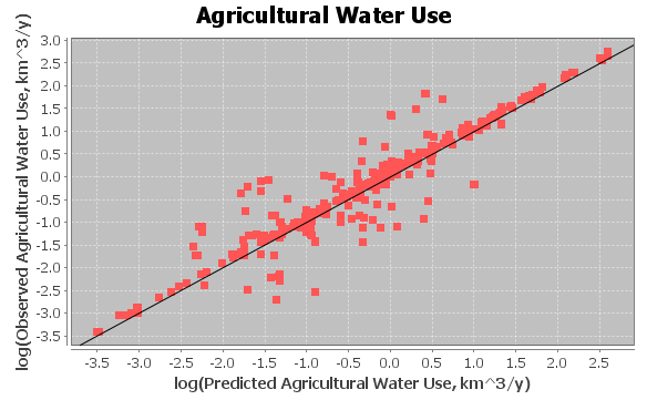
Plots of model predicted values vs. AQUASTAT observed values [7] for municipal, industrial, and agricultural water use from 1990 to 2011, superimposed against the predicted = observed line (perfect prediction). Municipal predictions appear to be most accurate (least deviation from the line), with larger deviations in industrial and agricultural predictions.
| Sector | R | ai | bi | Comments |
| Municipal | 0.9807 | 0.016 | 4.027 | Most accurate, variables for municipal demand (population, life expectancy, gdp/capita) good predictors of water demand. |
| Industrial | 0.9549 | 12.40 | 3.380 | Good accuracy, variables for industrial demand (energy consumption, gdp/capita) reasonable predictors of water demand. Smaller bi value than in municipal indicates that the point at which demand per consumer decreases is reached sooner in the industrial sector than in the municipal sector. |
| Agricultural | 0.9488 | 0.3106 | 0.031 | Good accuracy, variables for agricultural demand (agricultural land, temperature, precipitation) reasonable predictors of water demand. Influence of temperature on demand much greater than that of precipitation (a >> b) |
Table 1: Summary of behavior, accuracy, and observations of each model. R is the correlation coefficient between log(PRD) and log (OBS) over 1991-2011 data, used to measure how much variation in water demand is covered by variations in the predictive variables (R = 1 indicates perfect correlation). (ai,bi) are the coefficients for the model’s equations calibrated to 1970-1990 data, to produce usable equations from which predictions for water demand can be drawn.
Although the high R-values of the models indicate that most of the variation in water demand is covered by the model across various countries, the plots still show significant deviation between predicted and observed values with regard to the magnitude of a country’s water demand (several countries have water demand estimates three times as large as observed values). Consequently, rather than using predicted values directly, the relative growth rates of water demand in each sector were used to project changes in water demand, calculated from the original equations described in the model’s design.
Projections – Water Demand in 2030
In order to calculate future growth rates, projected values for the predictive variables from other studies were used:
- Population, from UN [6]
- Gross Domestic Product, from USDA [10]
- Life Expectancy, from UN [6]
- Total Energy Consumption, from EIA [11]
- Temperature, from World Bank [4]
- Precipitation, from World Bank [4]
Water demand growth rates by sector were projected from 2013 to 2030, and the total percent change from 2013 to 2030 were calculated. In total, there was sufficient data to fully analyze 167 countries, and the percent changes by sector and totals are displayed below:
| Industrial | Municipal | Agriculture | Total | |
| Decline | 29 | 66 | 66 | 80 |
| 0% – 10% Increase | 35 | 30 | 103 | 76 |
| 10% – 20% Incr. | 36 | 35 | 20 | 27 |
| 20% – 30% Incr. | 38 | 9 | 7 | 13 |
| 30% – 40% Incr. | 31 | 19 | 4 | 6 |
| Over 40% Incr. | 18 | 22 | 9 | 6 |
Table 2: Number of countries experiencing decline, 0%-10%, 10%-20%, 20%-30%, 30%-40%, and >40% increase in water demand from 2013 to 2030, by sector.
Observations
While there any many small scale observations to be made from the model’s results, at a global scale there is much diversity in water demand changes. With regards to geography, there are general regions experiencing larger water demand increases than others, but none of these regions are contiguous; many countries demonstrate changes in water demand that differ greatly from those of its immediate neighbors, in both sector composition and magnitude.
Furthermore, the diversity also appears to be independent of generalized classifications of development; varying levels of existing activity, expansion, and development in each of the three sectors across countries result in an total change of water demand that seems only loosely dependent of any single measure of development. There exist countries that are experiencing any level of water demand changes at every level of development, such income, as sorted by the World Bank’s income classifications:
| Lower | Lower-Mid. | Middle | Upper-Mid. | High | |
| Decline | 6.3% | 12.8% | 27.7% | 41.9% | 34.7% |
| 0% – 10% Increase | 37.5% | 48.7% | 41.0% | 34.9% | 53.1% |
| 10% – 20% Incr. | 21.9% | 23.1% | 19.3% | 14.0% | 6.1% |
| 20% – 30% Incr. | 21.9% | 5.1% | 3.6% | 2.3% | 4.1% |
| 30% – 40% Incr. | 9.4% | 5.1% | 2.4% | 0.0% | 2.0% |
| Over 40% Incr. | 3.1% | 5.1% | 6.0% | 7.0% | 0.0% |
Table 3: Percent of countries per World Bank income group in each level of water demand increase.
Recommendations
Though the exact numerical results of the model are not to be taken as a precise forecast of the future but rather as approximate and relative trends, Mission 2017 recommends certain considerations to make in future studies on water demand. Based on the model’s results, water demand trends vary widely by sector and short-range geography, and Mission 2017 suggests that total water demand can only be understood when investigated at a small-scale and by distinct sectors, in which more specific and well-defined sector divisions contribute to greater accuracy. Such specificity lends itself to a clearer identification of the consumer and level of development with regards to water use efficiency for each sector, which enables a more accurate forecast of water demand than those generated from generalized definitions. Mission 2017’s own sector divisions (municipal, industrial, agricultural) and interpretations should be considered a minimum in specificity, and future investigations should attempt to further subdivide these sectors.
However, developing such smaller-scale and sector-specific models is currently unreasonable as there is little data available with which to test models against. At the time of the study, water withdrawals by country were typically measured only once per decade per sector, making the investigation impossible at the country scale. Mission 2017 recommends that international organizations such as the UN Food and Agriculture Organization require countries to make more frequent measurements of water withdrawal by sector, and lead greater efforts for compiling, formatting, and sharing such data to enable the development of more accurate water demand models.
Conclusions
The results of the model indicate the complex nature of water demand patterns. Many countries demonstrate changes in water demand that differ greatly with those of its neighbors, in both composition and magnitude. To overcome the looming issue of water scarcity, it necessary to take into consideration not just the unequal distribution of water resources, but the unequal distribution of water demand. While some regions are not in immediate danger of water scarcity, it is only through the acknowledgement of these distinct distributions and the cooperation of countries that water security can be attained worldwide. Finally, with over half the world’s countries experiencing growth in water demand in the face of constant water supply [7], water scarcity will only become an increasingly severe problem without dedicated worldwide efforts towards more efficient water use.
Mission 2017 acknowledges that the issue of water scarcity is multidisciplinary and cannot be solved by single approach. Mission 2017 presents a diverse series of political, economic, and engineering solutions spanning all three sectors of water use in order to realize the necessary cooperation and technological changes for achieving global water security.
References
1. Strzepek, K., Schlosser, A., Gueneau, A., Gao, X., Blanc, E., Fant, C., Rasheed, B., & Jacoby, H. (2012, Dec). Modeling Water Resource Systems under Climate Change: IGSM-WRS. Retrieved from http://dspace.mit.edu/bitstream/handle/1721.1/75774/MITJPSPGC_Rpt236.pdf?sequence=1
2. Gassert, F., Landis, M., Luck, M., Reig, P., & Shiao, T. (2013, Jan). Aqueduct Global Maps 2.0. Retrieved from http://pdf.wri.org/aqueduct_metadata_global.pdf
3. FAO. (1990). Water and soil requirements. Retrieved from http://www.fao.org/docrep/U3160E/u3160e04.htm
4. World Bank. (2013). World Bank Open Data. Retrieved from http://data.worldbank.org
5. EIA. (2013). International Energy Statistics. Retrieved from http://www.eia.gov/cfapps/ipdbproject/IEDIndex3.cfm?tid=44&pid=44&aid=2
6. United Nations Department of Economics and Social Affairs. (2013). World Population Prospects: The 2012 Revisions. Retrieved from http://esa.un.org/wpp/index.htm
7. FAO. (2013). AQUASTAT. Retrieved from http://www.fao.org/nr/water/aquastat/main/index.stm
8. EIA. (2013, Jul 25). Industrial Sector Energy Consumption. Retrieved from http://www.eia.gov/forecasts/ieo/industrial.cfm
9. FAO (2009, Oct). Global agriculture towards 2050. Retrieved from http://www.fao.org/fileadmin/templates/wsfs/docs/Issues_papers/HLEF2050_Global_Agriculture.pdf
10. USDA Economic Research Service. (2013, Oct 28). Real Historical and Projected Gross Domestic Product (GDP) and Growth Rates of GDP. Retrieved from http://www.ers.usda.gov/datafiles/International_Macroeconomic_Data/Baseline_Data_Files/ProjectedRealGDPValues.xls
11. EIA. (2013, Jul 25). International Energy Outlook 2013. Retrieved from http://www.eia.gov/forecasts/ieo/
